
Blog
Comparison between euclidean 4dimensional electromagnetism and common electromagnetism
20/05/2014 22:50
Comparison between euclidean 4dimensional electromagnetism and common electromagnetism
In this article I compare the equations for euclidean 4dimensional electromagnetism whit the equations for standard electromagnetism and introduces a way to do calculations in euclidean 4dimensionell elektromagnetism whit ordinary concentretic ring magnetic fields.
Constants: µ0=4π10-7Vs/(Am) c=2,99792458¤108m/s ϵ0=8,8542¤10-12As/(Vm)
Where µ0 is the magnetical constant , ϵ0 is the electrical constant and c is the lightspeed in the Aether (vacuum).
µ0c2=1/ϵ0
B¤x=Byz-Bzy=By¤x+Bz¤x
B¤y=Bzx-Bxz=Bz¤y+Bx¤y
B¤z=Bxy-Byx=Bx¤z+By¤z
Bx¤y=-Bxz Bx¤z=Bxy
By¤x=Byz By¤z=-Byx
Bz¤x=-Bzy Bz¤y=Bzx
Where B¤x is the classical (ringformed) magnetic field in the x-direction , B¤y is the classical (ringformed) magnetic field in the y-direction , B¤z is the classical (ringformed) magnetic field in the z-direction , Bx¤y is the classical magnetic field in the y-direction from currents flowing in x-direction , Bx¤z is the classical magnetic field in the z-direction from currents flowing in x-direction , By¤x is the classical magnetic field in the x-direction from currents flowing in y-direction , By¤z is the classical magnetic field in the z-direction from currents flowing in y-direction , Bz¤x is the classical magnetic field in the x-direction from currents flowing in z-direction , Bz¤y is the classical magnetic field in the y-direction from currents flowing in z-direction.
Bxy=µ0∫jxdy Bxz=µ0∫jxdz
Byx=µ0∫jydx Byz=µ0∫jydz
Bzx=µ0∫jzdx Bzy=µ0∫jzdy
ρ0=(d3Q)/(dxdydz)
jx=ρ0vx=(d2I)/(dydz)
jy=ρ0vy=(d2I)/(dxdz)
jz=ρ0vz=(d2I)/(dxdy)
Where vx is the x-component of the velocity , vy is the y-component of the velocity , vz is the z-component of the velocity , Q is the electrical charge and I is the current , ρ0 is the charge density , jx is the x-component of the current density , jy is the y-component of the current density , jz is the z-component of the current density , Bxy is the magnetic field (straight field lines) in the y-direction from currents flowing in x-direction , Bxz is the magnetic field (straight field lines) in the z-direction from currents flowing in x-direction , Byx is the magnetic field (straight field lines) in the x-direction from currents flowing in y-direction , Byz is the magnetic field (straight field lines) in the z-direction from currents flowing in y-direction , Bzx is the magnetic field (straight field lines) in the x-direction from currents flowing in z-direction , and Bzy is the magnetic field (straight field lines) in the y-direction from currents flowing in z-direction.
Euclidean 4dimensional electromagnetism (correct theory)
Bxct=μ0∫jxcdt Byct=μ0∫jycdt Bzct=μ0∫jzcdt
Esx/c=μ0∫(ρ0vt)dx Esy/c=μ0∫(ρ0vt)dy Esz/c=μ0∫(ρ0vt)dz
vx2+vy2+vz2+vt2=c2 c=(vx;vy;vz;vt)
jx2+jy2+jz2+(ρ0vt)2 ρ0c=(jx;jy;jz;ρ0vt)
(dx)2+(dy)2+(dz)2+(cdt)2=(cdT)2=(ds4)2
ds4=cdT=(dx;dy;dz;cdt)
Where vt is the velocity in the time dimension , ds4 is the smallest possible distance 4vector , dT is the smallest possible true time interval , dt is the smallest possible coordinate time interval , dx is the smallest possible distance vector in the x-direction , dy is the smallest possible distance vector in the y-direction , dz is the smallest possible distance vector in the z-direction , Bxct is the magnetic field in the time dimension from currents flowing in x-direction , Byct is the magnetic field in the time dimension from currents flowing in y-direction , Bzct is the magnetic field in the time dimension from currents flowing in z-direction , Esx/c is the electrostatic field/c in the x-direction , Esy/c is the electrostatic field/c in the y-direction and Esz/c is the electrostatic field/c in the z-direction.
Ex=vtEsx/c+∫(dEsx/(cdT))cdt-vyByx-∫(dByx/dT)dy-vzBzx-∫(dBzx/dT)dz=vtEsx/c+∫(dEsx/(cdT))cdt+vyBy¤z+∫(dBy¤z/dT)dy-vzBz¤y-∫(dBz¤y/dT)dz
Ey=vtEsy/c+∫(dEsy/(cdT))cdt-vxBxy-∫(dBxy/dT)dx-vzBzy-∫(dBzy/dT)dz=vtEsy/c+∫(dEsy/(cdT))cdt-vxBx¤z-∫(dBx¤z/dT)dx+vzBz¤x+∫(dBz¤x/dT)dz
Ez=vtEsz/c+∫(dEsz/(cdT))cdt-vxBxz-∫(dBxz/dT)dx-vyByz-∫(dByz/dT)dy=vtEsz/c+∫(dEsz/(cdT))cdt+vxBx¤y+∫(dBx¤y/dT)dx-vyBy¤x-∫(dBy¤x/dT)dy
Ect=vxBxct+∫(dBxct/dT)dx+vyByct+∫(dByct/dT)dy+vzBzct+∫(dBzct/dT)dz
E2=Ex2+Ey2+Ez2+Ect2 E=(Ex;Ey;Ez;Ect)
U=∫Exdx+∫Eydy+∫Ezdz+∫Ectcdt
Where E is the electric field , and Ex is the x-component of the electric field , Ey is the y-component of the electric field , Ez is the z-component of the electric field , and Ect is the electric field component in the time dimension , and U is the scalar electrical potential.
As you sees from this theory it exists two totally different principles to construct time (zero point) energy converters , the first principle is anti lenz induction; you only uses the magnetic field that gives the induction while the magnetic fieldt that gives the lenz law is removed or better yet reversed so that the induction increases its own cause (devices that uses this principle; anti lenz unipolar, anti lenz synchron, anti lenz asynchron , corbino effekt MEG , SEG(searl effect generator)?). The other principle is based on the fact that the electrostatic field is a function of the time velocity of the charges and that particles whit space velocity gets lower time velocity , so that around a circuit an electrostatic field is present when it goes a current trough it even if it is the same amount of positive as negative elementary charges in the circuit and even if the current is constant and neither circuit nor observer is in motion (to get the phenomenon to be used for energy production the current must be a function of time (alternating current)so you get an alternating field)(devices that uses this principle for energy production: tesla MEG, ark of the Covenant, Great Pyramid(when it was in operation (it is possible that the ark of the Covenant was the central time (zero point) energy converter that powered it.)),wardenclyffe tower (maybe in combination whit tesla MEG). Devices that uses this principle to change their masses: UFO inertial damper and hyperdrive and stargates (these howewer whit direct current to get a constant very strong negative electrical potential to reduce the mass and cancel the inner potential of the matter to acces hyperspace)(positive potential at the recieving stargate.(more about this in Electrogravitation , Supplement to euclidean 4dimensional electromagnetism and electrogravitation and The hyperspace theory.)(SEG is possibly using this principle for inertial dampening)
(It is possible that SEG uses both principles for energy production or uses anti lenz induction for energy production and electrostatic field because of high current-speeds for inertial dampening).
Classical electromagnetism (wrong theory)
I will here present the equations for classical electromagnetism in integral and component form and show the errors that makes them useless to use to construct time (zero point) energy converters. I will mark correct parts of the theory whit green , completely wrong parts whit red and approximations whit purple
Esx=∫(ρ0/ϵ0)dx Esy=∫(ρ0/ϵ0)dy Esz=∫(ρ0/ϵ0)dz
( the formulas above is only valid when the charges stands still( in space dimensions))
Ex=∫(ρ0/ϵ0)dx+vyB¤z+∫(dB¤z/dT)dy-vzB¤y-∫(dB¤y/dT)dz=∫(ρ0/ϵ0)dx+vy(Bxy-Byx)+∫(d(Bxy-Byx)/dT)dy-vz(Bzx-Bxz)-∫(d(Bzx-Bxz)/dT)dz=∫(ρ0/ϵ0)dx-vyByx-∫(dByx/dT)dy-vzBzx-∫(dBzx/dT)dz+vyBxy+∫(dBxy/dT)dy+vzBxz+∫(dBxz/dT)dz==∫(ρ0/ϵ0)dx+vyBy¤z+∫(dBy¤z/dT)dy-vzBz¤y-∫(dBz¤y/dT)dz+vyBx¤z+∫(dBx¤z/dT)dy-vzBx¤y-∫(dBx¤y/dT)dz
Ey=∫(ρ0/ϵ0)dy-vxB¤z-∫(dB¤z/dT)dx+vzB¤x+∫(dB¤x/dT)dz=∫(ρ0/ϵ0)dy-vx(Bxy-Byx)-∫(d(Bxy-Byx)/dT)dx+vz(Byz-Bzy)+∫(d(Byz-Bzy)/dT)dz=∫(ρ0/ϵ0)dy-vxBxy-∫(dBxy/dT)dx-vzBzy-∫(dBzy/dT)dz+vxByx+∫(dByx/dT)dx+vzByz+∫(dByz/dT)dz==∫(ρ0/ϵ0)dy-vxBx¤z-∫(dBx¤z/dT)dx+vzBz¤x+∫(dBz¤x/dT)dz-vxBy¤z-∫(dBy¤z/dT)dx+vzBy¤x+∫(dBy¤x/dT)dz
Ez=∫(ρ0/ϵ0)dz+vxB¤y+∫(dB¤y/dT)dx-vyB¤x-∫(dB¤x/dT)dy=∫(ρ0/ϵ0)dz+vx(Bzx-Bxz)+∫(d(Bzx-Bxz)/dT)dx-vy(Byz-Bzy)-∫(d(Byz-Bzy)/dT)dy=∫(ρ0/ϵ0)dz-vxBxz-∫(dBxz/dT)dx-vyByz-∫(dByz/dT)dy+vxBzx+∫(dBzx/dT)dx+vyBzy+∫(dBzy/dT)dy==∫(ρ0/ϵ0)dz+vxBx¤y+∫(dBx¤y/dT)dx-vyBy¤x-∫(dBy¤x/dT)dy+vxBz¤y+∫(dBz¤y/dT)dx-vyBz¤x-∫(dBz¤x/dT)dy
The purple formulas above is only perfectly valid for stillstanding(in space) charges (an approximation , because of this approximation you misses the possibility of time (zero point) energy converters of the tesla MEG type (ark of the Covenant))
The green formulas is correct and is the same as in euclidean 4dimensional electromagnetism
The red formulas is completely wrong and not valid at all (Because of thes formulas it has been believed that lenz law is unavoidable and that time (zero point) energy converters of anti lenz induction type is impossible)
Esx is the electrostatic field in the x-direction according to classical electromagnetism , Esy is the electrostatic field in the y-direction according to classical electromagnetism , and Esz is the electrostatic field in the z-direction according to classical electromagnetism.
U=∫Exdx+∫Eydy+∫Ezdz
E2=Ex2+Ey2+Ez2 E=(Ex;Ey;Ez)
You have here missed an entire dimension
Conclusions
You have in classical electromagnetism completely missed the 4:th dimension and completely missed that it is motion trough the 4:th dimension that causes electrostatic fields you have also missed that this dimension the time dimension carries infinite amounts of energy that can be used to create heaven on earth. You don´t understand electric fields whit classical electromagnetism , whit euclidean 4dimensional electromagnetism you understand that electromagnetical fields is generated by charged particles that moves in the 4dimensional spacetime , magnetic fields by motion in space and electrostatic fields by motion in time! This is not understandable whit classical electromagnetism. Further so it becomes clear whit the staight magnetic field lines that the induction and the lenz law comes from different magnetic fields (in classical electromagnetism whit the concentretic ring magnetic fields you adds fields from currents in different directions and believe that they become equivalent and have the same properties altough they really are different fields and don´t have the same properties (It is on this way we missed the anti lenz induction)) and that is therefore possible to construct time (zero point) energy converters based on anti lenz induction. Further euclidean 4dimensional electromagnetism explains where the extra energy comes from; from the time dimension. (that the classical electromagnetismen have completely missed)
I hope that this article together whit the rest of my work should make you starting to use my equations instead of classical electromagnetism so that we can reshape the world into an utopian science fiction similiar paradise whit help of the time dimension.
(God vas the ancient name for the time dimension , that the ark of the Covenant was in contact whit God in reality means that the ark of the Covenant was a very powerful time (zero point) energy converter).
Artificial gravitation
20/05/2014 22:32
Artificial gravitation
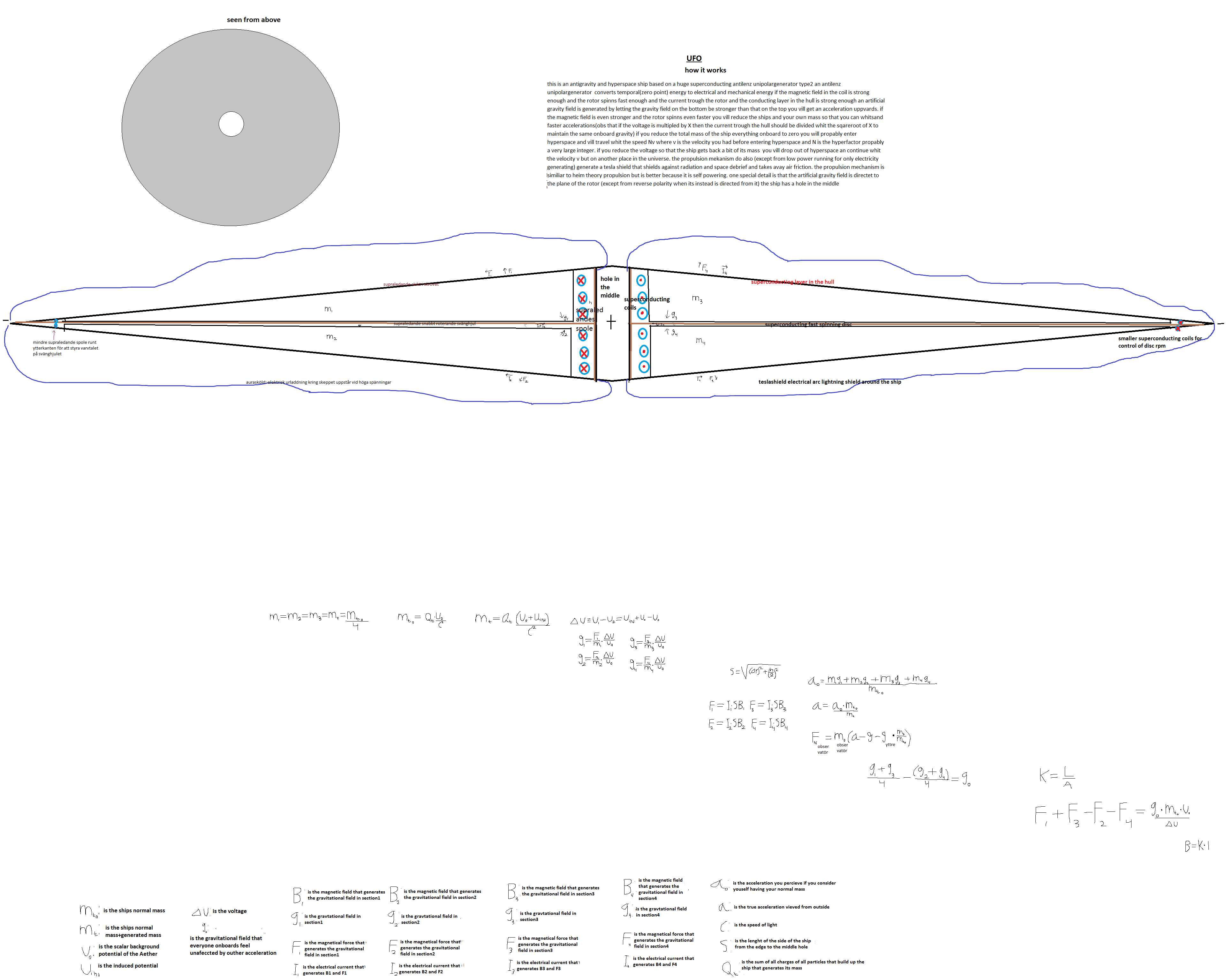
Gravitation is in reality no force but occurs of the reason that force and reaction force not fully take each other out because of the mass of one of the particles have been changed because of induced potential. All forces are outhermost of electromagnetic nature. Here comes the equation for gravity g0=F1ΔU/(m0tU0) where g0 is the acceleration that the system experiences when it is considered to have normal mass F1 is the force that generates the field, ΔU is the voltage between the points where force and counterforce acts, m0t is the total normal mass of the system, U0 is the backgroundpotential of the Aether. You can also calculate g that is the true acceleration that the system experiences g=F1ΔU/(mtU0) where mt=m0t(Uind+U0)/U0 where mt is the systems total mass and Uind is the average induced potential for the system.
The formulas is derived in this way F1=-F2 F1=m01a1 , F1=m02a2 m1=m01(Uind1+U0)/U0 m2=m02(Uind2+U0)/U0
Frest=m1a1+m2a2= m01a1(Uind1+U0)/U0+ m02a2(Uind2+U0)/U0= F1(Uind1+U0)/U0+ F2(Uind2+U0)/U0= F1Uind1/U0+F1+ F2Uind2/U0+F2= F1Uind1/U0-F1 Uind2/U0=F1(Uind1-Uind2)/U0=F1ΔU/U0 g= Frest/ mt= F1ΔU/(mtU0) and Uind=(∑m0nUindn)/m0t and Frest=m0tg0=mtg
Where Frest is the gravitational force (lacks reaktion force) m1 is the mass of particle1, m2 is the mass of particle2, F1 is the force on particle1
F2 is the force on particle2 (and also the reaction force to F1 ), Uind1 is the induced potential at particle1, ), Uind2 is the induced potential at particle2, ), Uindn is the induced potential at particle n, m0n is the normal mass of particle n, m01 is the normal mass of particle1, m02 is the normal mass of particle2
These equations explains how UFOs can fly in normalspace and explains why you are’nt weightless in a UFO. The equations can be used to construct artificial gravitational fields. F1 and F2 is forces of electromagnetic nature.
The Pioneer maser signal anomaly: Possible confirmation of spontaneous photon blueshifting
20/05/2014 22:20
1
The Pioneer maser signal anomaly:
Possible confirmation of spontaneous photon blueshifting
P. A. LaViolette
April 2005
Physics Essays, volume 18(2), 2005
The Starburst Foundation, 1176 Hedgewood Lane, Niskayuna, NY 12309
Electronic address: gravitics1@aol.com
Abstract
The novel physics methodology of subquantum kinetics predicted in 1980 that photons
should blueshift their frequency at a rate that varies directly with negative gravitational
potential, the rate of blueshifting for photons traveling between Earth and Jupiter having
been estimated to average approximately 1.3 ± 0.65 X 10⁻¹⁸ s-1, or 1.1 ± 0.6 X 10⁻¹⁸ s-1 for
signals traveling a roundtrip distance of 65 AU through the outer solar system. A proposal
was made in 1980 to test this blueshifting effect by transponding a maser signal over a 10
AU round-trip distance between two spacecraft. This blueshift prediction has more recently
been corroborated by observations of maser signals transponded to the Pioneer 10
spacecraft. These measurements indicate a frequency shifting of approximately 2.28 ± 0.4
X 10-18 s-1 which lies within 2σ of the subquantum kinetics prediction and which cannot be
accounted for in terms of known forces acting on the craft. This blueshifting phenomenon
implies the existence of a new source of energy which is able to account for the luminosities
of red dwarf and brown dwarf stars and planets, and their observed sharing of a common
mass-luminosity relation.
Résumé
La nouvelle théorie de la physique du cinétique subquantique avait prévu en 1985 que les photons
devraient se déplacer vers le bleu à un rythme qui varie directement avec le potentiel de la gravité
négative. Le taux de déplacement de photons vers le bleu entre la Terre et Jupiter est estimé être
approximativement (1.3 ± 0.65) X 10-18 s-1, ou de (1.1 ± 0.6) X 10-18 s-1 pour le chemin allerretour
de signaux d'une distance de 65 AU à travers la région extérieure du système solaire. Une
proposition a été faite en 1980 afin de vérifier l'effet du déplacement vers le bleu par un signal
maser de transpondeur sur une distance aller-retour entre deux engins spatiaux. Cette prédiction fut
corroborée par l'observation des signaux maser de transpondeur vers le vaisseau spatial du Pionnier
10. Ces mesures indiquent un décalage de fréquence approximativement de 2.28 ± 0.4 X 10⁻¹⁸ s-1,
qui se trouve en dessous de 2σ de la prévision de la cinétique subquantique et qui n'est pas expliqué
en terme des forces connues agissant sur le vaisseau. Ce phénomène de déplacement vers le bleu
suggère l'existence d'une nouvelle source d'energie qui explique les luminositiés des étoiles naines
rouges et naines brunes, des planètes, et leur partage d'une relation de luminosité masse commune.
_______________________________________________________________________
Key words: time and frequency, planetary and deep space probes, gravitational wave detectors
and experiments, energy conservation violations, subquantum kinetics, nonequilibrium and
irreversible thermodynamics, genic energy, frequency blueshifting, mass-luminosity relation,
planets and stars
2
1. INTRODUCTION
During the past 30 years, 2.1 GHz maser signals have been transmitted to the Pioneer 10 and
Pioneer 11 spacecraft and coherently transponded back to Earth, the frequency shift of the received
signal being used to determine the recessional velocity of the spacecraft for purposes of navigation.
However, Anderson et al.(1, 2) report that when the computed velocity is compared to the velocity
predicted by orbital models, a discrepancy is found, even after adjustments are made for all known
forces that might act on the spacecraft. They find a frequency blueshift residual that increases
linearly with time, or in direct proportion to the increase in the line-of-sight distance to the
spacecraft.
If interpreted as a Doppler effect, this residual implies the presence of an anomalous force
accelerating the craft toward the Sun which Anderson et al. calculate to be 8.7 ± 1.3 X 10⁻⁸ cm/s2.
Although, as is discussed below, when the propulsive effects of on-board thermal radiation sources
are taken into account, this decreases to a residual acceleration of 6.85 ± 1.3 X 10⁻⁸ cm/s2. If
interpreted as an anomalous acceleration, the effect is perplexing since most plausible forces, such
as gravity, decrease rapidly with distance whereas the Pioneer apparent acceleration remains
relatively constant with time. Moreover, an anomalous acceleration of similar magnitude does not
appear to be acting on the planets, given that their orbital periods experience no similar secular
change within the accuracy of current determinations.(2)
It is here suggested that this linear blueshifting is instead due to a continual spontaneous
increase in photon frequency which local photons normally undergo, but which until now has
passed unnoticed due to the small size of the effect. For example, the rate of frequency shifting
implied by the Pioneer 10 data, 2.28 ± 0.4 X 10⁻¹⁸ s-1, would be many orders of magnitude smaller
than rates detectable in the laboratory. Over a laboratory photon travel distance of 100 meters this
would amount to a frequency change of one part in 1024, as compared with the U.S. Naval
Observatory hydrogen maser clock system which is stable to only one part in 1015 for a one day
integration time.
This alternative interpretation explains in a straightforward manner the anomalous frequency
shifting of the Pioneer spacecraft signals by means of a phenomenon that has no effect on planet
orbits. But, more importantly, the observed effect was predicted over a decade before the
announced discovery of the Pioneer anomaly, being first mentioned in 1980 and described in later
publications to be a necessary consequence of the subquantum kinetics physics methodology.(3 - 7)
In 1980, the author had proposed an experiment that could test for this blueshifting effect by
transponding a maser signal between two spacecraft separated by a distance of 5 AU (e.g.,
positioned at 1 AU and 6 AU) and the return signal being measured to determine whether its
frequency had increased at the predicted average rate of μ ~ 1.3 ± 0.65 X 10⁻¹⁸ s-1. The beam was
to be modulated with regularly spaced pulses whose period in the return beam could be compared
to the initial pulse period to determine the relative movement of the craft. In this way the Doppler
component of the maser signal's frequency change would be known so that a check could be made
3
for the presence in the beam of a nonDoppler frequency shift residual.
At that time in 1980, the author had contacted Frank Estabrook at the Jet Propulsion Laboratory
(JPL), one of John Anderson's colleagues, and inquired about the possibility of conducting such a
space-based experiment.(8) But at that time his group was mainly interested in using spacecraft
maser signal residuals as a way of detecting gravity waves and testing the predictions of general
relativity.(9 - 11) Nevertheless this discussion gave assurance that a maser signal traveling over the
course of a 10 AU roundtrip journey would accrue a frequency shift large enough to be marginally
measurable above the background noise that would be present in the return signal due to
disturbance by the solar plasma. A description of this proposed maser signal experiment was
submitted for journal publication in 1980 and was later documented in expositions of subquantum
kinetics published in 1985 and 1994.(3, 4, 6)
Subquantum kinetics predicts that the magnitude of the blueshifting rate varies linearly with the
magnitude of the local ambient gravitational potential. Hence, compared with the value in the Earth's
environs (1.3 X 10⁻¹⁸ s-1), for signals transponded from Earth to a spacecraft such as Pioneer 10
located at 65 AU, it predicts a slightly lower blueshifting rate of μ ~ 1.1 ± 0.6 X 10⁻¹⁸ s-1. This
prediction is strikingly close the observed Pioneer 10 value, being about half of the observed rate.
If the Pioneer spacecraft tracking anomaly remains unexplained by more conventional phenomena,
such as waste heat radiation, then the observed anomalous frequency shift may be a legitimate
verification of this previously documented subquantum kinetics blueshifting prediction.
2. THE PHOTON BLUESHIFTING PREDICTION
Subquantum kinetics postulates that the electric and gravitational field potentials that form
photons, subatomic particles, and zero-point energy fluctuations, arise as inhomogeneities in an
underlying, all-pervading plenum whose constituents engage in well-defined nonequilibrium
reaction-diffusion processes which are represented by a nonlinear equation system; see Ref. [4 - 6]
for a full explanation. The electric field potential solutions of this equation system exhibit
nonconservative as well as conservative behavior depending upon the value of the ambient
gravitational potential, ϕg, relative to a critical potential value ϕgc; see Figure 1.(4, 6) Hence in
subquantum kinetics, perfect energy conservation, photon energy remaining constant with the
passage of time, is the exception rather than the rule, occurring only when this underlying reaction
system operates at its critical threshold. For example, the system would operate at this threshold of
marginal stability in regions of space bounding the fringes of galaxies where the ambient gravity
potential approaches the critical threshold value; i.e., where ϕg = ϕgc. In regions where ϕg < ϕgc,
such as in a galaxy's gravity well, supercritical conditions would prevail, dictating a progressive
increase in photon energy with the passage of time and spontaneous photon blueshifting. In
intergalactic regions of space where gravity potential attains positive values relative to the critical
threshold, ϕg > ϕgc, subcritical conditions would prevail, dictating a progressive decrease in photon
energy with the passage of time and photon redshifting. Photons traveling from distant galaxies
4
Figure 1. Hypothetical intergalactic gravity potential field and its creation of
supercritical and subcritical regions.
would be subject to predominantly subcritical conditions along their flight path and hence would
undergo a redshift scaling in proportion to their distance or time of travel. This "tired-light" effect
model has been shown to make a good fit to cosmological redshift data on a variety of cosmology
tests.(12 - 14) The nonconservative energy behavior predicted by subquantum kinetics does not
contradict the first law of thermodynamics, since the First Law strictly applies to closed systems,
whereas the nonequilibrium subquantum reactions postulated in subquantum kinetics instead
constitute an open system.
The absolute value of the gravitational potential is important in that as a control factor it
determines not only whether a photon will be in an energy gaining or energy losing mode, but also
the degree to which photons will depart from perfect energy conservation, i.e., the rate at which
photon energy will either increase or decrease. Subquantum kinetics represents the time
dependence of photon energy by the following general relation:
E(t) = E0eμt , (1a)
where μ = -α(ϕg – ϕgc). (1b)
E0 representing the photon's initial energy, E(t) its energy after time t, and μ its rate of energy
change. Coefficient μ varies linearly with the value of the ambient (negative) gravitational potential
ϕg as indicated in (1b), where ϕgc is the critical threshold gravity potential and α is a proportionality
constant having units of time/area (e.g., s/cm2).
In order to simplify the above equation, let us assign a value of zero to the critical threshold ϕgc.
Then, negative gravity potential values (ϕg < 0) relative to the critical threshold zero point dictating
supercritical, energy amplifying conditions and positive values (ϕg > 0) dictating subcritical, energy
damping conditions, but, in addition, ϕg determines the rate at which a photon's energy is expected
to change over time. Alternatively, (1a) may be expressed as:
5
ν(t) = ν0e-αϕgt , (2)
where ν0 is the photon's initial frequency and ν(t) its frequency at time t. This frequency shifting
effect may also be expressed as:
dν
dt = μν = -αϕgν (3)
Note that this frequency shift is a new effect that is not predicted by standard physics theories
and should therefore not be confused with the better known gravitational frequency shift
phenomenon which arises due to the difference in ambient gravity potential between the region of
photon emission and region of photon reception. The hypothesized phenomenon would occur even
when there is virtually no net change of gravity potential, as in the case of maser signals
transponded over a round-trip path. Also unlike the gravitational redshift, the proposed
phenomenon should have no observable effect on photon emission processes, since many hours are
required before a photon has accumulated a frequency shift large enough to be observed, and even
then the amount is very slight. So, this effect should not be observable in stellar spectra. Over a
distance of 10 kpc, photons traveling from a distant star would accumulate a blueshift of
approximately 0.3 km/s, an amount that would be insignificant in comparison to shifts attributable
to the conventional gravitational frequency shift phenomenon.
To provide a realistic cosmology, the reaction-diffusion system postulated as the basis of
subquantum kinetics must operate very close to its threshold of marginal stability in an initially
subcritical state prevailing during the era prior to the emergence of quanta. This allows the reaction
system to spawn material particles out of the prevailing zero-point energy fluctuation background.
Moreover by designing the reaction system so that the parameter regulating system criticality is
identified with gravity potential, the reaction system is able to generate supercritical conditions in the
vicinity of materialized particles and celestial bodies (i.e., in gravity wells) thereby ensuring that
their forms are sustained over time. As a consequence of this cosmology, photons traveling in
supercritical regions within celestial bodies and in their environs would gradually blueshift. The
manner in which a photon's field potential would evolve over time is specified by (1a) above.
To take the next step and make a quantitative prediction of the rate of photon blueshifting that
would be expected for a given gravity potential value, one must constrain the reaction system model
with observation. Since the subquantum level is inherently unobservable, its variables being hidden
from us, in order to constrain the constants in (1b) we are left to use physical observations such as
bolometric luminosities for the Sun and planets. This may be done by adjusting parameter α and
the value assumed for the galactic gravity background potential, ϕgal, to give a realistic value of μ as
a function of ϕg such that the resulting energy blueshifting rate yields the correct bolometric
luminosities for these celestial bodies. This modeling was done in earlier discussions of the photon
blueshifting effect,(3,5) and is reviewed and updated in the next section. Once this modeling was
done and the subquantum kinetics photon blueshifting prediction was accordingly defined, the
resulting blueshifting rate then emerged as a testable prediction, one that could later be checked
6
through the proposed maser signal experiment. As is shown below, the Pioneer spacecraft data
later confirmed this prediction.
Understandably, subquantum kinetics takes a different approach than that used in general
relativity. For example, its gravitational effects are not theorized to result from a warping of spacetime.
Rather, effects such as gravitational attraction or repulsion, gravitational time dilation, and the
bending of starlight by celestial bodies are effects that emerge as consequences of the postulated
subquantum reactions.(14) The postulated subquantum reaction processes also predict that electric
and gravitational potential fields should be coupled at all energies, a result that has been verified.(4,
14) Note that the proposal that gravity potential controls the rate of photon energy change, itself
presupposes the existence of a link between gravitational and electric potential fields. Hence
subquantum kinetics qualifies as a unified field theory.
3. EARLY MODELING OF THE AMPLIFICATION COEFFICIENT
Equation (3) predicts that the energy reservoir within a celestial body should spontaneously
generate excess energy ("genic" energy) through this photon blueshifting effect at a rate equal to
the product of the blueshifting rate coefficient μ and the reservoir's total heat capacity, H:
Lg = dE/dt = μH ~ –αϕg
–
CM
–
T, (4)
where H is given approximately as the product of the body's average specific heat –
C , mass M, and
average internal temperature
–
T.(4, 6) This blueshifting effect is expected to act in the same way on all
photons regardless of their frequency. In this model, heat capacities Hi are estimated for each body
based on the body's mass, and on a reasonable estimate of its average internal temperature and
specific heat. Furthermore, a planet's average internal gravity potential is modeled to be
approximately ϕg = 2 ϕ0 + ϕsun + ϕgal , where ϕ0 is its surface gravity potential, ϕsun is the gravity
potential contribution from the Sun at the planet's heliocentric distance, and ϕgal is an additional
background factor contributed by the Galaxy as a whole relative to the local intergalactic
background potential. When variables α and ϕgal are properly chosen, (4) is found to account for
most or all of the internal energy output observed to come from the interiors of the planets Earth,
Jupiter, Saturn, Uranus, and Neptune.(5, 6) Genic energy luminosities Lg estimated for the Sun,
planets, and Sirius B are presented in Table I along with the values for ϕ,
–C
, M, and
–
T, for
comparison to observed luminosities. This table is similar to that presented in an earlier publication
of this prediction, Table II of Ref. 5, but with slightly revised values for μ, calculated by assuming α
= 2.62 X 10⁻³² s/cm2 and ϕgal = -4 X 1013 cm2/s2.
The photon blueshifting predicted for the Earth environs is so small as to be undetectable in the
laboratory, but it should be large enough to be measurable over interplanetary distances. Using the
modeled values for α and ϕgal, it is possible to make a testable prediction of the blueshifting rate
one would expect to find in interplanetary space. That is, expressing (3) as μ = –αϕg = –α(ϕgal +
7
Table I: Modeling Parameters and Intrinsic Luminosities for the Sun, Planets and Sirius B.
Star or
Planet
M
(g)
R
(cm)
ϕ0
(cm2/s2)
r
(cm)
ϕsun
(cm2/s2)
ϕgal
(cm2/s2)
–μ
(s-1)
–C
(erg/g/°K)
–T
(°K)
Lg
(erg/s)
Li
(erg/s)
Sun 1.99 (33) 6.96 (10) -1.91 (15) - - - - - - -4.0 (13) 1.00 (-16) 2.1 ± 0.8 (8) 9.5±3 (6) 4.0±2.5 (32) 3.90 (33)
Mercury 3.30 (26) 2.44 (8) -9.02 (10) 6.00 (12) -2.21 (13) -4.0 (13) 1.63 (-18) 1.26±0.5 (7) 2 ± 1 (3) 1.4±0.9 (19) - - -
Venus 4.87 (27) 6.05 (8) -5.37 (11) 1.12 (13) -1.19 (13) -4.0 (13) 1.39 (-18) 1.26±0.5 (7) 2.5±1 (3) 2.1±1.4 (20) - - -
Earth 5.98 (27) 6.38 (8) -6.25 (11) 1.50 (13) -8.87 (12) -4.0 (13) 1.31 (-18) 1.26±0.5 (7) 2.5±1 (3) 2.5± 1.5 (20) 4.0±0.2 (20)
Moon 7.35 (25) 1.74 (8) -2.82 (10) 1.50 (13) -8.87 (12) -4.0 (13) 1.28 (-18) 1.26±0.5 (7) 2 ± 1 (3) 2.4± 1.5 (18) 7.0±0.5 (18)
Mars 6.44 (26) 3.39 (8) -1.27 (11) 2.36 (13) -5.62 (12) -4.0 (13) 1.20 (-18) 1.26±0.5 (7) 2 ± 1 (3) 2.0±1.2 (19) 3 ± 2 (19)
Jupiter 1.90 (30) 6.92 (9) -1.83 (13) 8.06 (13) -1.65 (12) -4.0 (13) 2.05 (-18) 1.18±0.5 (8) 9 ± 5 (3) 4.1±2.6 (24) 3.4±0.3 (24)
Saturn 5.69 (29) 5.73 (9) -6.62 (12) 1.48 (14) -8.99 (11) -4.0 (13) 1.42 (-18) 8.1±3.0 (7) 6 ± 3 (3) 3.9±2.5 (23) 8.6±0.1 (23)
Uranus 8.74 (28) 2.57 (9) -2.27 (12) 2.97 (14) -4.47 (11) -4.0 (13) 1.18 (-18) 3.8 ± 1.5 (7) 4 ± 2 (3) 1.6±1.0 (22) 0.3±0.4 (22)
Neptune 1.03 (29) 2.53 (9) -2.72 (12) 4.65 (14) -2.85 (11) -4.0 (13) 1.17 (-18) 3.6 ± 1.5 (7) 4 ± 2 (3) 1.7± 1.1 (22) 3.3±0.4 (22)
Pluto 6.60 (26) 2.90 (8) -1.52 (11) 4.65 (14) -2.85 (11) -4.0 (13) 1.06 (-18) 1.26±0.5 (7) 2 ± 1 (3) 1.8±0.7 (19) - - -
Sirius B 2.10 (33) 5.6 (8) -2.5 (17) - - - -5.0 (17) -4.0 (13) 1.3 (-14) 3.0 ± 1.5 (6) 1±0.8 (6) 8.3± 5.3 (31) 1 ± 0.2 (32)
a The numbers in brackets represent powers of 10. The values for the model parameters listed in Table I were
determined as follows. For all celestial bodies considered here, the gravity potential is calculated relative to a
background value of ϕgal = -4 × 1013 cm2/s2, which includes the gravity potential contribution of the Galaxy, galaxy
cluster, and supercluster. The average internal gravity potential ϕg for the Sun is estimated to be two times its
surface potential, 2ϕ0 , plus ϕgal , where ϕo = -Mkg/R, kg being the gravitational constant and R being the Sun's
radius. The internal gravity potentials for the planets, including the Earth and Moon, are calculated as:
ϕg = 2ϕo + ϕsun + ϕgal , where ϕsun = -Mkg/r represents the contribution from the Sun's gravity potential field at
the planet's heliocentric distance, r. The ϕg values for the planets are dominated primarily by the Galactic
component. In the case of Sirius B, the potential is calculated to be ϕg = 2ϕ0.
The values for μ– are calculated as μ– = –αϕg, with α = 2.62 × 10⁻³² s/cm2. The value for α is chosen such that
the calculated genic energy luminosity for the Sun is normalized to 0.1 L, which should be allowable even in light
of the results of the Sudbury Neutrino Observatory solar neutrino experiment.
Values adopted for the average specific heats and internal temperatures are the same as those given in reference [4]
with the exception of the temperature for Sirius B. For a reasonable fit to be made to the observed bolometric
luminosity (Li ) for Sirius B, we must choose an average temperature for its interior that is an order of magnitude
lower than temperatures normally modeled for its core. This is permissible if it is assumed to have a deep
convective layer capable of easily conveying heat to its surface. The Li data point for Sirius B is taken from F.
Paerels, et al. Ap. J.329 (1988): 849-862.
MG/r), where M is the Sun's mass, r is the maser photon's heliocentric distance in AU, and G is
the gravitational constant, and choosing α = 2.62 X 10⁻³² s/cm2 and ϕgal = -4 X 1013 cm2/s2, the
interplanetary blueshifting rate at a given distance r from the Sun is given as:
μ = (1.05 +
0.22
r
) X 10-18. (5)
According to (5), a maser signal making a round-trip journey between the Earth and a spacecraft
located at 65 AU would blueshift at the average rate of μ ~ 1.05 X 10⁻¹⁸ s-1, the second term in the
equation making a negligible contribution. This falls close to blueshifting rates later observed for
signals transponded back from Pioneer 10 and 11.
Equation (5) predicts that the rate of blueshifting should be greater at times when the maser
signal transponded between the Earth and the spacecraft has a trajectory that takes it near the Sun.
8
Hence the blueshifting incurred over the round-trip signal path between the Earth and spacecraft
would be expected to fall to a minimum when the spacecraft was at solar opposition and to rise to a
sharp peak when the spacecraft approached solar conjunction, at which point the maser signal
would at one point reach a minimum heliocentric distance of r = 5 X 10⁻⁴ AU. The modeled α and
ϕ values predict that this annual effect should cause the cumulative round-trip blueshift to vary by
about ±2%. Anderson et al. do report an annual variation in the magnitude of the Pioneer
spacecraft anomalous acceleration which is similarly strongly peaked at solar conjunction and falls
to a minimum at solar opposition. However, the annual variation they observe is much larger, on the
order of ±30% of the average blueshifting rate; see Figure 1 of Ref. 15 or Figure 14 of Ref. 2.
They propose that this variation may be due to unexplained modeling errors in the Earth's orbital
orientation or in the accuracy of the planetary ephemeris. If such is the case, until they are
corrected, these modeling error uncertainties will mask the annual variation predicted by (5).
Due to the uncertainty in knowing the true value of the Galactic gravity potential in the Sun's
vicinity, ϕgal is used here as a modeling variable whose value, together with that of coefficient α, is
chosen so that (4) makes a best overall fit to the bolometric luminosities of the Sun and planets. In
an earlier paper describing this predicted blueshifting effect,(5) these variables were instead modeled
as α = 5.23 X 10⁻³² s/cm2 and ϕgal = -2 X 1013 cm2/s2, for their fit to observed luminosity data,
which specified the blueshifting coefficient as μ = (1.05 + 0.46
r
) X 10-18. The revised values
reflect a fit to new luminosity data which requires a lower genic energy contribution to the Sun's
bolometric luminosity. Nevertheless, at large r these two models make essentially the same
prediction, deviating by < 0.6% at r = 40 AU. Hence in regard to the Pioneer maser data, both
models predict essentially the same average blueshifting rate for μ since this data spans heliocentric
distances ranging from ~20 to 65 AU where the second term is very small. Future space based
experiments carried out in the inner solar system region around 1 AU should determine whether the
second term in (5) is properly modeled.
Note that the earlier published derivation of μ was done with no foreknowledge of the Pioneer
Effect since the latter had not been discovered at that point. Also adjustments of this μ value made
in the present paper were made solely with the intent to arrive at an adequate fit to the solar and
planetary luminosity data. For example, this new fit makes a much lower genic energy prediction
for the Sun, which accords with the updated lower main sequence M-L data discussed below. This
new adjustment of the values of α and ϕgal took into account no consideration of the Pioneer Effect
results. Moreover, as noted above, the earlier and present model predictions for μ make the same
quantitative prediction for the Pioneer data. Hence the subquantum kinetics blueshifting prediction
stands as a valid a priori prediction.
The modeled value of ϕgal = -4 X 1013 cm2/s2 is low compared to what standard theories
predict for the Galactic contribution to the local gravity potential. However, it is nevertheless
consistent with observation. For example, Olling and Merrifield have modeled the Milky Way's
rotation and found that the available data is best fit if the galactocentric distance for the Sun is set at
9
r0 = 7.1 ± 0.4 kpc with a solar orbital velocity of v0 = 184 ± 8 km/s.(16 - 19) These values are
smaller than those of other Galaxy dynamics models, which assume r0 = 8.5 kpc and v0 = 220
km/s. However, a smaller value for r0 is corroborated by the best primary measurements which
place the galactocentric distance at 7.2 ± 0.7 kpc.(20) Olling and Merrifield estimate a mass for the
Galaxy's central bulge of Mb ~ 8.3 X 10⁹ M, based on a bulge k-band luminosity of Lb ~ 1.5 X
1010 L and a mass-luminosity ratio of 0.55.(19) For a galactocentric distance of r0 = 7.1 kpc, this
would contribute a gravity potential of -5 X 1013 cm2/s2 to the solar vicinity. Gerhard(21) estimates
a larger mass for the galactic bulge of 1.3 X 10¹⁰ M which predicts a larger contribution of -7.8 X
1013 cm2/s2. The Galaxy's disc makes a smaller contribution to the local gravitational potential.
Kuijken and Gilmore have determined that the matter column density within 1.1 kpc of the galactic
plane is Σ1.1 kpc = 71± 6 M/pc2 which includes the halo contribution as well.(22) Integrating this
contribution out to a distance of 7 kpc yields a gravity potential contribution to the solar vicinity of
2πrGΣ1.1 kpc = -4.2 ± 0.4 X 1013 cm2/s2. Hence including the larger estimate for the bulge
contribution, the total Galactic gravity potential contribution to the solar vicinity would be Δϕgal ~
-12± 3 X 1013 cm2/s2.
To obtain ϕgal, the Galactic gravity potential contribution Δϕgal must be added to the value of
the intergalactic background potential which according to subquantum kinetics is positive relative to
ϕgc, the zero critical point value; see Figure 1. An average value for the intergalactic background
potential may be obtained from the cosmological redshift as: ϕ–int = H0/α, where H0 is the Hubble
constant expressed in seconds-1. As mentioned earlier, subquantum kinetics interprets the
cosmological redshift as a tired-light effect, a spontaneous loss of energy specified by (1) where ϕg
is in this case positive relative to ϕgc. This yields an average intergalactic background potential that
is approximately the same magnitude as the solar system value except opposite in sign with respect
to the critical threshold zero point value. Taking H0 = 72 ± 10 km/s /Mpc and α = 2.62 X 10⁻³²
s/cm2, we obtain ϕ–int = 8.9 ± 1.2 X 1013 cm2/s2. Adding to this Δϕgal would yield ϕgal = -3 ± 3
X 1013 cm2/s2. which is close to the -4 X 1013 cm2/s2 value we are assuming.
Subquantum kinetics predicts that over great distances the gravity potential field should taper
off to a plateau in intergalactic space, each galaxy's field being effective n its own gravity well
locale.(4, 6). This is similar in many respects to MOND (Modified Newtonian Dynamics) which is
an observationally based approach that allows the plateau in galaxy orbital velocities to be modeled
without introducing assumptions about outlying hidden mass.(23 - 25) In subquantum kinetics,
however, this field tapering emerges as a prediction of the theory itself which requires that potential
fields be slightly nonsolenoidal, that at large r the gravity potential should be less negative than
would be expected from the Newtonian 1/r relation. Translated into more familiar terms, this would
be similar to summing a galaxy's potential at a given point with the potential produced by a
distributed background of "virtual antimatter" which presents a negative mass density (positive ϕg).
At increasing distances from a galaxy, an increasing volume of this negative mass would be
encompassed within the sphere defined by that radial distance and this would have the effect of
10
increasingly screening the galaxy's positive mass, progressively reducing its potential from what
would normally be predicted by a Newtonian 1/r law. Thus if this distributed background is taken
to be equivalent to a negative mass density of ρ = -10-30 g/cm3, which approximates the negative of
the intergalactic mass density, then a Galaxy of mass 5 X 10¹⁰ M would have its gravity field
entirely screened at a galactocentric distance of 3 million light years at which point the gradient of
its potential field would be zero. To satisfy MOND, a more rapid attenuation of the gravity field
would be required, MOND requiring that attenuation of the gravitational force begins to be
noticeable when the field's gravitational acceleration has diminished below a critical threshold of a0
= 10-8 cm/s2.
The idea of a truncated range for gravity is consistent with the observation of Tifft that
neighboring and distant galaxies do not appear to dynamically interact with one another.(26)
Moreover others have argued on theoretical grounds that a range limit to gravity would avoid
problems associated with space having an arbitrarily high or infinite value for its gravity potential
contribution from extragalactic sources.(27) A finite range for gravity would be problematic for
models that predict galaxy formation through gradual accretion of a primordial gas cloud.
However, this is not a problem with nonstandard creation models such as subquantum kinetics
which predict galaxy formation through continuous matter creation in a galaxy's core and gradual
outward growth with later stage formation of spiral arms, a scenario supported by Hubble telescope
observations of distant galaxies.(14)
4. ASTROPHYSICAL CONSEQUENCES OF PHOTON BLUESHIFTING
The existence of photon blueshifting and the resulting production of "genic energy" would have
significant implications for astrophysics in that genic energy would make a major contribution as a
stellar power source, supplementing nuclear fusion and gravitational accretion. For example, (4)
predicts that red dwarfs, brown dwarfs, and planets should be powered exclusively by genic energy
and should share a common mass-luminosity relation of approximately L ∝ M2.7 ± 0.9; see ref. (5)
for details. In fact, the jovian planets are seen to lie along the lower main sequence stellar massluminosity
relation which, using the data of Harris et al.,(22) is of the form L ∝ M2.76 ± 0.15; see
Fig. 2.(5, 6) The brown dwarfs LP 944-20, G 196-3B, and GL 229B(29-32) also are found to lie
close to this line confirming earlier predictions.(4 - 6) These correspondences provide strong
confirmation for the subquantum kinetics blueshifting prediction since on standard theory they
must be passed off as pure coincidence.
Between 0.4 M and 0.6 M (L ≈ 0.025 - 0.05 L), the mass-luminosity relation becomes
somewhat scattered and less well defined. It is in this transition region where the upper main
sequence mass-luminosity relation begins, the M-L relation changing to a steeper slope of L ∝ M4;
(dashed line in Fig. 2). This transition would signify the point where nuclear burning begins to
make a noticeable contribution, supplementing genic energy production. When projected to lower
masses, the upper main sequence M-L relation is found to intersect the lower main sequence M-L
11
Figure 2. The mass-luminosity coordinates of the jovian planets shown
in relation to the lower main sequence stellar mass-luminosity relation.
The M-L coordinates for the recently discovered brown dwarfs (LP 944-20,
G196-3B, and GL 229B) also are found to lie close to this line.
relation at around 0.4 M. But the lower main sequence relation data trend does not entirely
disappear until a somewhat higher mass is reached, possibly around 0.6 to 0.7 M. The luminosity
gap evident between the lower and upper main sequence relations would indicate the additional
contribution provided by nuclear fusion, nuclear burning providing a progressively larger share of a
star's total radiated energy as stellar mass increases.
In this mass range of 0.2 to 0.5 M, where the lower main sequence transitions to the upper
main sequence, the lower log M-log L relation gradually bends downward to a slightly lower slope.
12
Figure 3. A nonlinear curve fit to red dwarf mass-luminosity data.
The circle in the upper right hand corner is the indicated value when
the regression is projected up to 1 M.
This may be seen in Figure 3, which plots a nonlinear regression curve fit made to log M and log L
data for red dwarfs in the mass range 0.06 M through 0.6 M. The plotted values are listed in
Table II. In cases where the cited sources list visual magnitudes instead of luminosity values,
bolometric luminosities are calculated using the models of Baraffe, et al. by knowing the spectral
classifications of the respective stars.(33) This downward bend, or "plateau," has also previously
been noted by Henry et al. who have attributed the effect partly to a deepening of a star's convective
region as stellar mass increases.(34)
When extrapolated upward to 1 M, the resulting regression line projects a bolometric
luminosity of 0.16 ± 0.07 L for the Sun. Subquantum kinetics, then, predicts that around 16% of
the Sun's energy should be of non-nuclear genic origin with the remaining majority being supplied
by nuclear fusion.(35) While the Sudbury Neutrino Observatory solar neutrino experiment results
have resolved the mystery as to why other solar neutrino experiments had previously reported low
solar neutrino fluxes, the proposal that fusion may provide only 84± 7 % of the Sun's energy is
nevertheless tolerable in view of the range of uncertainty of stellar fusion models.
If the existence of the photon blueshifting phenomenon is acknowledged, all stellar evolution
models will need to be revised. As described in previous publications, genic energy is also able to
account for high-luminosity white dwarfs and X-ray stars and can explain how certain quasars are
13
Table II: Masses and Luminosities of Low Mass Stars
Star log M—
M
log L—
L
Ref. Star log M—
M
log L—
L
Ref.
GL 22 A -0.44 -1.64 [a] GL 747A -0.67 -2.25 [b]
GL 22 C -0.89 -2.57 [a] GL 747B -0.70 -2.32 [b]
GL 65 A -0.99 -2.99 [b] GL 748A -0.42 -1.80 [c]
GL 65 B -1.00 -3.07 [b] GL 748B -0.72 -2.00 [c]
GL 166 C -0.75 -2.20 [a] GL 791.2B -0.90 -3.15 [b]
GL 234 A -0.69 -2.36 [b] GL831 A -0.54 -2.20 [b]
GL 234 B -0.99 -3.08 [b] GL 831 B -0.79 -2.66 [b]
GL 473 A -0.84 -2.91 [b] GL 860 A -0.57 -2.07 [b]
GL 473 B -0.88 -2.91 [b] GL 860 B -0.76 -2.40 [b]
GL 570 B -0.25 -1.30 [b] GL 866 A -0.92 -2.98 [b]
GL 570 C -0.42 -1.52 [b] GL 866 B -0.94 -3.03 [b]
GL 623 A -0.46 -1.71 [a] GL 866 C -1.03 -3.24 [b]
GL 623 B -0.94 -2.64 [a] YY Gem A -0.22 -1.22 [b]
GL 644 A -0.38 -1.63 [b] YY Gem B -0.22 -1.32 [b]
GL 644 Ba -0.46 -1.65 [b] GJ 1245 A -0.89 -2.94 [a]
GL 644 Bb -0.50 -1.77 [b] GJ 1245 C -1.13 -3.44 [a]
GL 661 A -0.42 -1.69 [b] CM Dra a -0.64 -2.25 [b]
GL 661 B -0.43 -1.7 [b] CM Dra b -0.67 -2.29 [b]
LP 944-20 -1.22 -3.80 [d]
[a] T. J. Henry, O. G. Franz, L. H. Wasserman, G. F. Benedict, P. J. Shelus, P. A. Ianna,
J. D. Kirkpatrick, and D. W. McCarthy, Jr., Ap. J. 512, 864 (1999).
[b] X. Delfosse, T. Forveille, D. Ségransan, J.-L. Beuzit, S. Udry, C. Perrier, and M.
Mayor, Astron. Astrophys. 364, 217 (2000).
[c] G. F. Benedict, B. E. McArthur, O. G. Franz, L. H. Wasserman, T. J. Henry, T.
Takato, I. V. Strateva, J. L. Crawford, P. A. Ianna, D. W. McCarthy, et al., A. J. 121,
1607 (2001).
[d] C. G. Tinney, MNRAS 296L, 42 (1998); C. G. Tinney and I. N. Reid, MNRAS 301,
1031 (1998).
able to power themselves in the absence of nearby gas and dust, a recognized problem for black
hole theory.(4 - 6, 14) Moreover genic energy can account for phenomena such as stellar pulsation,
novae, and supernovae. That is, since photon blueshifting can feed back to increase a star's internal
temperature and heat capacity which in turn increases the rate at which energy is produced, this
inherent nonlinearity can ultimately lead to instability.
In an earlier 1985 paper, the author pointed out that the photon blueshifting rate estimated for
photons traveling in the solar system was approximately the same magnitude as the energy
attenuation rate needed to account for the cosmological redshift, but of opposite sign;(4, 6) and more
recently, discoverers of the Pioneer Effect have similarly noted that the blueshifting anomaly has a
magnitude comparable to H0.(2) In fact, the revised estimate of the Pioneer data blueshifting rate
discussed below (2.28 ± 0.4 X 10⁻¹⁸ s-1) is exactly equal in magnitude to the negative Hubble
constant value, the subquantum kinetics prediction being about half this amount. In the context of
subquantum kinetics, this correspondence between the predicted Pioneer maser signal blueshifting
rate and the cosmological redshifting rate would be an indication that the value of the gravitational
14
potential for regions of space within galaxies does not depart far below the critical threshold, just as
the intergalactic value of the gravitational potential does not depart far above the critical threshold.
This is consistent with the requirement in subquantum kinetics that the underlying subquantum
reaction-diffusion system operates very close to the threshold of marginal stability, and that it had
resided predominantly in a subcritical state during the period preceding the emergence of matter in
supercritical regions. If the subquantum reactions had not initially operated near its critical
threshold, they would have had little chance of spawning material particles out of the zero-point
energy fluctuation background.
5. ADJUSTING THE PIONEER BLUESHIFTING ANOMALY DATA FOR
UNMODELED THERMAL EFFECTS
As mentioned above, the magnitude of the Pioneer anomalous acceleration effect reported by
Anderson et al. should be reduced to 82% of its value to take into account the propulsive effects
due to waste heat radiated from the spacecraft. For example, Scheffer, Katz, and Murphy have
suggested that a portion of the apparent anomalous acceleration acting on the Pioneer spacecraft
may be due to thermal radiation striking the anti-solar side of its antenna coming from the passive
radiators used to cool the spacecraft's electronics, from its RTG power unit, and from various other
sources.(36 - 38) Scheffer's model predicts that the thrust from these thermal sources should have
declined by 11.8% from "Period I" (~10/1988) through "Period III" (~7/1995) due to a decline in
available spacecraft power and changes in the types of experiments being carried out. Instead, a
much smaller rate of decrease in acceleration is seen. The SIGMA WLS values computed for the
anomalous Pioneer 10 acceleration, listed in Table I of Ref. [2], indicate a decrease of 2% from
Period I to Period III, whereas the CHASMP WLS values indicate a decrease of 4.1% over this
same time period. Averaging these two values, it appears that the spacecraft's acceleration decreased
by about 3.05 ± 1% over this period.(39) Consequently, if this 3% decrease is entirely due to the
above unmodeled heating effects, these effects would be responsible for at most
(3.05 ± 1%)/11.8% = 26 ± 9% of the anomalous "acceleration." Although (5) indicates there
should be some degree of decrease in μ as the spacecraft's heliocentric distance progressively
increases, this decline would be very slight, only 0.15% during the above mentioned interval.
Anderson et al., however, maintain that such unmodeled thermal effects account for a much
smaller percentage of the anomalous apparent acceleration,(2,40-42) and include a bias correction of
only -0.55 X 10⁻⁸ cm/s2 to take into account the propulsive effect of heat radiated from the RTG
unit; see Table II of Ref. [2]. They find no variation in Pioneer 10's computed acceleration over a
certain period from mid 1992 to mid 1998 and offer this as evidence that the unmodeled thermal
effects play a minor role. However, since their trend line was calculated from data that included the
±30% annual variation described above, their regression line slope will very much depend on which
dates they pick to begin and end their trend-line average. Consequently, a 3% secular decline may
still be present in their data yet be masked by the much larger irregular annual variation. Hence a
15
negative conclusion in regard to a decline in spacecraft acceleration is unwarranted.
The above discussion of Scheffer's thermal effects model, suggests that the anomalous
acceleration value of 8.7 ± 1.3 X 10⁻⁸ cm/s2 reported by Anderson, et al. should be reduced by the
additional amount of 1.86 ± 1.3 X 10⁻⁸ cm/s2, i.e., 0.26 × (8.7 + 0.55) × 10-8 -0.55 × 10⁻⁸ cm/s2,
to give an unexplained residual of 6.85 ± 1.3 X 10⁻⁸ cm/s2. Expressed in terms of photon
blueshifting, this residual would amount to 2.28 ± 0.4 X 10⁻¹⁸ s-1, which comes strikingly close to
the blueshifting rate predicted by subquantum kinetics.
6. GALILEO RANGING MEASUREMENTS.
If the unexplained frequency shift phenomenon is a Doppler shift produced by an anomalous
force acting on the spacecraft, as Anderson et al. have suggested, then one should observe a
corresponding change in the spacecraft's range relative to the Earth. That is, the spacecraft should
be found to be closer than would otherwise be expected. If the frequency shift instead arises
spontaneously as a nonDoppler blueshift affecting only the transponded maser signal, as
subquantum kinetics predicts, then one should expect to find no corresponding change in spacecraft
range. Unfortunately, the Pioneer 10 and 11 spacecraft were not outfitted for ranging
measurements. So Anderson et al. attempted to check for the presence of ranging anomalies by
comparing the ranging and "Doppler shift" data received from the Galileo spacecraft. Ranging
measurements were made by modulating the outgoing maser beam with markers and observing the
time taken for a given marker to be transponded back to Earth. The Doppler shift measurements
were made by comparing the frequencies of the outgoing and incoming maser beams. Anderson et
al. claim that the marker timing measurements showed a decrease in spacecraft range approximating
the amount that would be expected if the anomalous blueshifting they observe in their Doppler shift
data were due to unmodeled forces acting on the spacecraft.(2) Consequently, they concluded that
the data did not favor the alternative explanation of spontaneous frequency blueshifting, which they
alternatively construe as the "time acceleration" hypothesis.
However, there are reasons for doubting their conclusion. For one thing, the data they used was
recorded relatively close to the Sun (1 to 5 AU) while the Galileo spacecraft was traveling from near
the Earth to Jupiter, a region where solar radiation pressure and solar plasma effects dominate the
measurements. By comparison, Anderson et al. began studying the Doppler signal data from the
Pioneer 10 and 11 spacecraft only after these spacecraft had surpassed a distance of 20 AU, at
which point solar radiation pressure acceleration had decreased to < 5 X 10⁻⁸ cm/s2. The same
measure of caution should be applied to the Galileo ranging and Doppler measurements, raising the
question as to the reliability of that data. In fact, Anderson et al. state that the solution they obtained
for the Galileo spacecraft Doppler measurement data was so highly correlated with solar pressure
and so complicated by mid-course orbital maneuvers that a standard null result could not be ruled
out. They also acknowledge that the signal-to-noise ratio on the incoming range signal was small,
requiring long integration times during which time the range of the spacecraft was constantly
16
changing at a rate of ~6 km/s. Additional uncertainty was introduced because the identification of
the code for the appropriate received ranging signal was inferred, sometimes with great difficulty,
from the orbit determination programs.
Moreover, as mentioned above, Anderson et al. question the accuracy of the solar system
modeling programs they used, speculating that modeling errors in these programs may be the cause
of the large unexplained annual variation observed in residual acceleration. In the case of Pioneer
10 and 11, as the spacecraft progressed from 40 AU to 70 AU, the maser signal path length varied
by a small percentage, about ±2%, due to distance variation arising from the movement of the Earth
about the Sun (±1 AU vs . 55 AU), yet their data charted a large annual variation of ±25%. By
comparison, Galileo's measurements were made 20 times closer to the Sun in the vicinity of 1 - 5
AU where the annual variation of the maser signal path length, relative to the total distance to the
spacecraft, was at least 25 times greater. In this near solar environment, the variable annual
component of the acceleration would have substantially exceeded the nonvarying component
making ranging determinations even more uncertain. Furthermore, when a maser signal passes
through the solar plasma, ranging measurements will experience a time delay, making the calculated
spacecraft distance abnormally large, whereas the transponded return signal used in making the
Doppler frequency comparison will experience a phase advance, making the calculated inferred
spacecraft distance abnormally small.
Although ranging data was also available from the Ulysses spacecraft, those measurements were
considered even less reliable than those from Galileo. In summary, the measurements that
Anderson et al. used to rule out the spontaneous photon blueshifting effect are, by their own
admission, fraught with difficulty. Hence their range change conclusion should be viewed with
caution.
If the Pioneer Effect is in fact due to a spontaneous change in photon energy, as subquantum
kinetics predicts and is not due to an anomalous force acting on the spacecraft, then it will be
necessary to adjust for this effect in Doppler tracking of spacecraft. For example, consider the
anomalous force of 8.7 X 10⁻⁸ cm/s2 which Anderson et al. suggest acts on the Pioneer 10
spacecraft. If this is imagined to be real and to have acted on the spacecraft for a full 30 years, then
navigators will place the craft's position 390,000 km closer to the Sun than if the force were believed
to be absent and the blueshifting due to a nonDoppler blueshifting effect. This is about the distance
from the Earth to the Moon, and could result in quite a large error if the nature of the blueshifting is
misjudged.
7. FUTURE EXPERIMENTS AND CONCLUSION
A definitive resolution of the issue of whether Doppler and ranging anomalies really exist may
have to await a future out-of-solar system spacecraft mission such as the Pluto/Kuiper mission
scheduled for launch around 2006 and which includes very sophisticated tracking technology. In
addition, as a result of efforts by Turyshev et al.,(43) the European Space Agency has suggested that
17
a new spacecraft experiment be launched into the outer solar system around 2015 to exclusively
test the Pioneer Effect. The experiment would be designed to characterize the properties of the
anomaly to an accuracy of at least two orders of magnitude below the anomaly's size.
Another possibility would be to make modifications to the Laser Interferometer Space Antenna
(LISA) so that it could detect the predicted effect. LISA, which is due to be launched in 2010,
involves three spacecraft placed in the Earth's solar orbit separated from one another by 5 million
kilometers to form three legs of a triangle with a phase-locked laser beam along each leg.(44)
Although the experiment is planned to be carried out fairly close to the Sun (~1 AU), solar plasma
has little effect on laser beam transmission, hence should not pose a problem. LISA will be able to
detect accelerations of as little as 10-13 cm/s2 (equivalent to a frequency shift rate of ~10-23 s-1),
which is about 105 times smaller than the predicted effect. However, the experiment is currently
being designed primarily for the purpose of detecting low frequency gravity waves in the milli Hz
frequency range and as such is not focused on detecting a "DC" effect similar to that produced by
the Pioneer anomaly, whether it be a constant accelerating force or a constant nonDoppler photon
blueshifting effect.(45)
However, it should be possible to check for the Pioneer effect. At 1 AU from the Sun, the
predicted genic energy effect is expected to blueshift each laser beam at the rate of 1.27 ± 0.7 ×
10-18 s-1, making the beam accumulate a frequency shift of 4.2 X 10⁻¹⁷ by the end of its 107 km
roundtrip. For a beam wavelength of 1 μm, (f = 3 X 10¹⁴ Hz), this would amount to a frequency
difference of Δf = 0.0127 Hz. The resulting interference pattern would move through one fringe
cycle every 1/Δf = 79 seconds toward the lower frequency reference laser. This effect would be the
same for each leg of the triangle regardless of each beam's orientation. LISA will be using
photodiode detectors having an interferometer fringe resolution of 4 X 10⁻⁵ λ/ Hz which would
allow this net fringe drift to be easily detected.
A nonDoppler frequency shift effect may be distinguished from Doppler shifts arising from
relative drifting of the spacecraft by modulating the laser beam with regularly spaced AM pulses or
polarization shift markers. Any change in the period of these time markers would indicate
exclusively the Doppler component of the frequency shift since the marker period would be
relatively immune to any change in laser frequency. If the laser transponder is instructed to return a
signal that is offset from the original laser frequency by twice the Doppler frequency shift, this
would effectively null out the Doppler component when the transponded signal is received back,
and would leave the photon blueshifting effect to appear in the data coming from each leg as the
primary fringe drift residual. If the Pioneer effect were instead due to an anomalous force pulling
spacecraft toward the Sun, it should accelerate all three LISA spacecraft at approximately the same
rate and hence would be expected to yield no net frequency shift effect.
It is hoped that the necessary design modifications will be made to LISA to allow a test to be
made of this important physical effect. As a follow-up to LISA, a similar experiment could later be
conducted closer to the Sun where the ambient gravity potential is more negative and where
18
subquantum kinetics predicts that higher blueshifting rates should be observed. Until these
experiments are carried out, the subquantum kinetics blueshifting prediction should provide a useful
alternative to consider in interpreting the Pioneer 10 and 11 tracking anomaly.
References:
[1] J. D. Anderson, P. A. Laing, E. L. Lau, A. S. Liu, M. M. Nieto, and S. G. Turyshev, Phys. Rev.
Lett. 81, 2858 (1998); Eprint arXiv:gr-qc/9808081.
[2] J. D. Anderson, P. A. Laing, E. L. Lau, A. S. Liu, M. M. Nieto, and S. G. Turyshev, Phys. Rev.
D 65, No. 082004 (2002); Eprint arXiv:gr-qc/0104064.
[3] P. A. LaViolette, "Do celestial bodies violate the energy conservation law?," manuscript
submitted in 1979 and 1980 for journal publicaton and later published in revised form in 1992
in Physics Essays; see reference [5].
[4] P. A. LaViolette, Int. J. Gen. Sys. 11, 329 (1985).
[5] P. A. LaViolette, Phys. Essays 5, 536 (1992); erratum: Phys. Essays 6, (1993).
[6] P. A. LaViolette, Subquantum Kinetics; The Alchemy of Creation, first edition (Starlane
Publications, Alexandria, VA, 1994), p. 135.
[7] P. A. LaViolette, Beyond the Big Bang (Park Street Press, Rochester, VT, 1995), p. 299.
[8] In their 2002 Physical Review paper [2], Anderson et al. mention that the anomalous
blueshifting effect in the Pioneer data first became noticeable in 1980, however, at that time they
were not sure that it was a real effect. It was not until about 1990, realizing that the anomaly
would not go away, that the JPL team concluded that the data should be more closely examined
[M. Nieto, private communication]. Thereafter the anomaly was mentioned publicly for the first
time at a 1994 conference and in that same year a serious study of the data was begun which
continued through 2002, with journal publications appearing in 1998 and 2002. So, my
communication with JPL suggesting the existence of such a blueshifting effect would predate
even the early stages of the discovery of this effect in the Pioneer maser data. When I contacted
F. Estabrook of JPL in 1980, he had indicated that they were unaware of any persistent
blueshift in spacecraft maser data.
[9] F. B. Estabrook and H. D. Wahlquist, Acta Astronautica 5, 5 (1978).
[10] J. W. Armstrong, R. Woo, and F. B. Estabrook, Ap.J. 230, 570 (1979).
[11] J. D. Anderson and F. B. Estabrook, J. Spacecraft and Rockets 16, 120 (1979).
[12] P. A. LaViolette, Ap. J. 301, 544 (1986).
[13] A. A. Ubachukwu and L. I. Onuora, Astrophys. Space Sci. 209, 169 (1993).
[14] P. A. LaViolette, Subquantum Kinetics, 2nd edition (Starlane Publications, Alexandria, VA,
2003), Chapter 7.
19
[15] S.G., Turyshev, J.D. Anderson, P.A. Laing, E.L. Lau, A.S. Liu, and M.M. Nieto, in
Gravitational Waves and Experimental Gravity, Proc. XVIII Moriond Workshop of the
Rencontres de Moriond, edited by J. Dumarchez and J. Tran Thanh Van (World Publishing,
Hanoi, 2000), pp. 481 - 486; Eprint arXiv:gr-qc/9903024.
[16] R.P. Olling and M.R. Merrifield, ASPC 136, 216 (1998); Eprint arXiv:astro-ph/9711157.
[17] R.P. Olling and M.R. Merrifield, Mon. Not. R. Astron. Soc. 297, 943 (1998); Eprint
arXiv:astro-ph/9802034.
[18] R.P. Olling and M.R. Merrifield, Mon. Not. R. Astron. Soc. 311, 361 (2000); Eprint
arXiv:astro-ph/9907353.
[19] R.P. Olling and M.R. Merrifield, Mon. Not. R. Astron. Soc. 326, 164 (2001); Eprint
arXiv:astro-ph/0104465.
[20] M.J. Reid, A.R.A.&A. 31, 345 (1993).
[21] O. Gerhard, Space Science Reviews 100, 129 (2002); Eprint arXiv:astro-ph/0203110.
[22] K. Kuijken and G. Gilmore, Ap.J. 367, L9 (1991).
[23] M. Milgrom, Ap.J. 270, 365 (1983).
[24] M. Milgrom, Ap.J. 270, 371 (1983).
[25] R. Brada and M. Milgrom, MNRAS 276, 453 (1995).
[26] W.G. Tifft, Ap. J. 211, 31 (1977).
[27] S.V.M. Clube, MNRAS 193, 385 (1980).
[28] D.L. Harris III, K.Aa. Strand and C.E. Worley, in Basic Astronomical Data (Univ. Chicago
Press, Chicago, 1963), p. 285.
[29] C.G. Tinney, MNRAS 296L, 42 (1998).
[30] C.G. Tinney and I.N. Reid, MNRAS 301, 1031 (1998).
[31] R. Rebolo, M.R. Zapatero Osario , S. Madruga, V.J.S. Bejar, S. Arribas, and J. Licandro,
Science 282, 1309 (1998).
[32] S.K. Leggett, D.W. Toomey, T.R. Geballe, and R.H. Brown, Ap.J. 517, L139 (1999).
[33] I. Baraffe, G. Chabrier, F. Allard, and P.H. Hauschildt, A&A 337, 403 (1998).
[34] T.J. Henry, O.G. Franz, L.H. Wasserman, G.F. Benedict, P.J. Shelus, P.A. Ianna, J.D.
Kirkpatrick, and D.W. McCarthy, Jr., Ap. J. 512, 864 (1999).
[35] In previous publications [4-7] the lower main sequence M-L relation had been assumed to
have a linear log-log plot in which case its upward projection indicated a luminosity of about
0.58 L. On this basis it had been proposed that ~58% of the Sun's energy was of nonnuclear,
genic energy origin. This has now been revised downward to 16% based on the new
data presented in Table II, which indicates that the relation bends down at its upper end.
[36] E.M. Murphy, Phys. Rev. Lett. 83, 1890 (1999); Eprint arXiv:gr-qc/9810015.
[37] J.I. Katz, Phys. Rev. Lett. 83, 1892 (1999); Eprint arXiv:gr-qc/9809070.
[38] L.K. Scheffer, 2001. Eprints arXiv:gr-qc/0107092; gr-qc/0108054.
20
[39] J.D. Anderson, P.A. Laing, E.L. Lau, A.S. Liu, M.M. Nieto, and S.G. Turyshev, Phys. Rev.
Lett. 83, 1893 (1999); Eprint arXiv:gr-qc/9906112.
[40] J.D. Anderson, P.A. Laing, E.L. Lau, A.S. Liu, M.M. Nieto, and S.G. Turyshev, Phys. Rev.
Lett., 83 1891 (1999); Eprint arXiv:gr-qc/9906113.
[41] J.D. Anderson, E.L. Lau, S.G. Turyshev, P.A. Laing, and M.M. Nieto, Mod.Phys.Lett. A17,
875 (2002); Eprint arXiv:gr-qc/0107022.
[42] In the cited references, Anderson et al. propose that the decline in computed acceleration from
interval I to interval III was somehow associated with a change in the spacecraft's spin rate,
although they do not explain how spin rate might induce this effect.
[43] S.G. Turyshev, M.M. Nieto, and J.D. Anderson, paper presented at 35th COSPAR Scientific
Assebly,' July 18-24, 2004, Paris, France; Eprint arXiv:gr-qc/0409117.
[44] (LISA) Laser Interferometer Space Antenna System and Technology Study Report, July 2000;
https://www.srl.caltech.edu/lisa/documents/sts_1.05.pdf.
[45] B.L. Schumaker, LISA team member, personal communication, April 2005.
Items: 10 - 12 of 79
